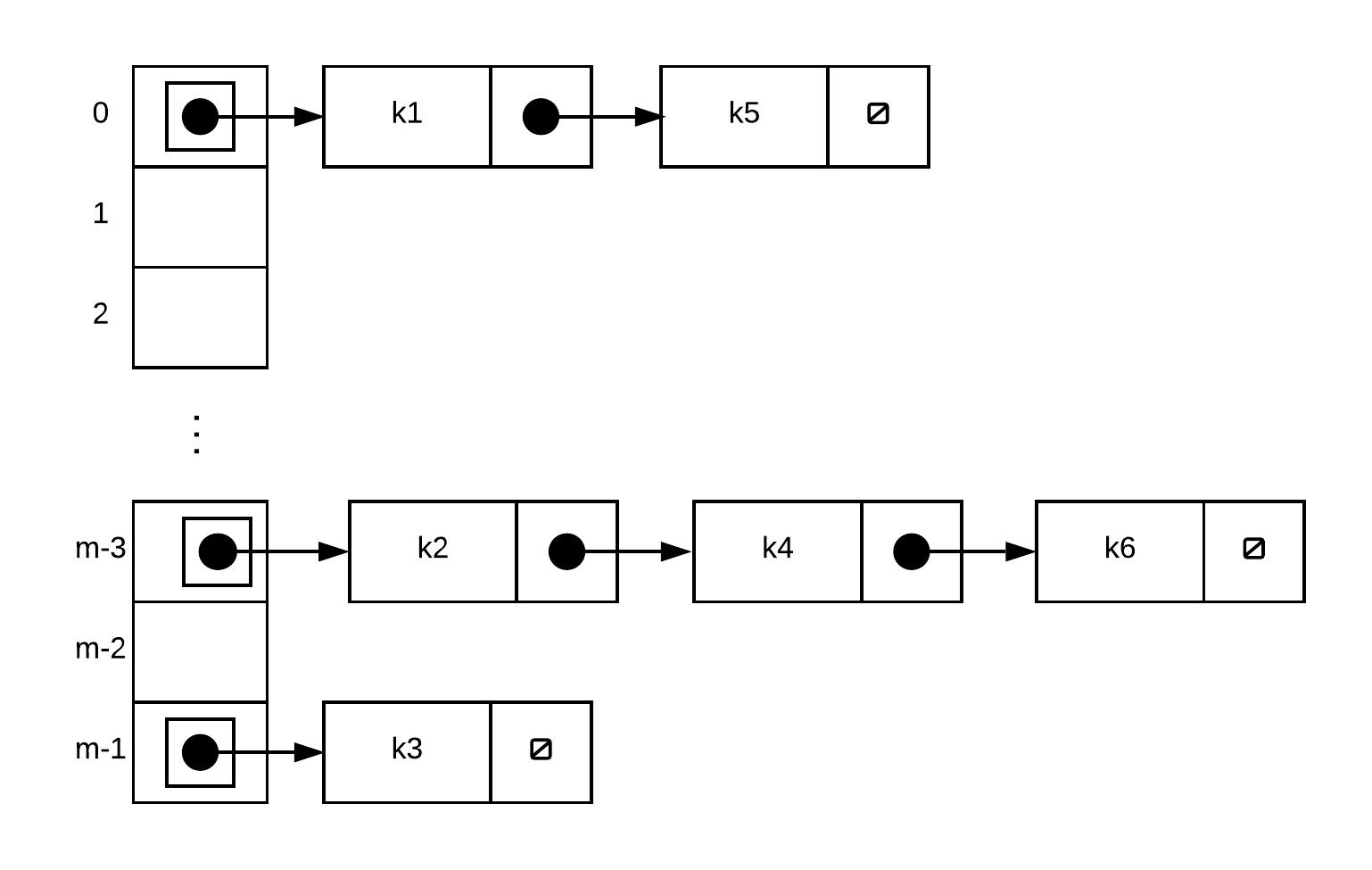
Chaining

At every location (hash index) in your hash table store a linked list of items. You only use as many nodes as necessary. Using Chaining the Table will not overflow as you can have as long a chain as you need. However, You will still need to conduct a short linear search of the linked list but if your hash function uniformly distributes the items, the list should not be very long.

For chaining, the runtimes depends on the load factor ($\lambda$) The average length of each chain is $\lambda$ . $\lambda$ is the number of expected probes needed for either an insertion or an unsuccessful search. For a successful search it is $1+ {\lambda \over 2}$ probes.

While it is possible for $\lambda >1$, it is generally not a great idea to be too much over. Your goal isn't to search long chains as that is very slow. The ability to have long chains is more of a safety feature... you should try to still have as short a chain as possible.

Chaining is a simple way of handling collisions. Instead of storing the key-value pair $(k,v)$ into the array (with capacity $m$) directly, chaining creates an array of linked lists, initially all empty.For each operation involving key$k$

• calculate $i=hashIndex(k,m)$
• perform operation (insert/delete/search) on the linked list at array[i]

Example

Suppose we were to have 6 keys $(k1,k2,k3,k4,k5,k6)$. The hash function returns as follows for these keys:

• $hashIndex(k1, m)==0$
• $hashIndex(k2,m)==m−3$
• $hashIndex(k3,m)==m−1$
• $hashIndex(k4,m)==m−3$
• $hashIndex(k5,m)==0$
• $hashIndex(k6,m)==m−3$

A table created using chaining would store records as follows (note that only key's are shown in diagram for brevity)

Worst case run time

insert(k,v) - cost to find the correct linked list + cost to search for k within the linked list, + cost to add new node or modify existing if k is found

search(k) - cost to find the correct linked list + cost to search for k within the linked list

delete(k) - cost to find the correct linked list + cost to search for k within the linked list + cost to remove a node from list

In each of the above cases, cost of to find the correct linked list is $\theta(1)$ assuming that the cost of calculating hash is constant relative to number keys. We simply need to calculate the hash index, then go to that location

The cost to add a node, modify a node or delete a node (once node has been found) is $\theta(1)$ as that is the cost to remove/insert into linked list given pointers to appropriate nodes

The cost to search through linked list depends on number of nodes in the linked list. At worst, every single key hashes into exactly the same index. If that is the case, the run time would be $\theta(n)$

Thus, the worst case run time is $\theta(n)$. In reality of course, the performance is signficantly better than this and you typically don't encounter this worst case behaviour. Notice that the part that is slow is the search along the linked list. If our linked list is relatively short then the cost to search it would also not take very long.

Average case run time

We begin by making an assumption called Simple Uniform Hash Assumption (SUHA). This is the assumption that any key is equally likely to hash to any slot. The question then becomes how long are our linked lists? This largely depends on the load factor $\lambda = n/m$ where n is the number of items stored in the linked list and m is the number of slots. The average run time is $\theta( 1 + \lambda)$